How Much Measurement Error is Too Much? Part I: Modelling Measurement Data

By R.K. Henderson, DuPont Photomasks Inc.

It is widely accepted in the electronics industry that measurement gauge error variation should be no larger than 10% of the related specification window. Process industries, such as chemicals and textiles, have operated for years without meeting this 10% criterion. This paper borrows a framework from the process industries for evaluating the impact of measurement error variation in terms of both customer and supplier risk (non-conformance and yield loss). In many circumstances the 10% criterion may be more stringent than is necessary. Part I discusses the relationship between measurement processes and production processes; Part II applies the resulting model to realistic process and measurement variations.

In the most general terms, this paper provides a theoretical basis for evaluating the relative magnitude of measurement process error and using measurement data to determine whether or not a specific product characteristic meets a supplied specification. Electronics-related industries have generally agreed that measurement error spread, generally defined as 3s of the measurement process, should be no larger than 10% of the allowable product specification window. To date, this 10% criterion has not been overly difficult to achieve, suggesting one reason why it is still widely accepted and communicated. In some sectors of the electronics industry, however, this criterion is finally receiving some resistance.

An example of such a situation is in the production of photomasks. Photomasks represent the first transformation of the circuit design concept into a physical entity; they essentially perform the role of the "mold" for the semiconductor. Features on the mask that do not meet the requested tolerances will generally transfer to the wafer, potentially leading to poor performance of the final circuitry.

Photomask manufacturers routinely evaluate feature size in terms of the critical dimension (CD), a measurement of one or more features of a targeted size. Accuracy of mask CDs has become increasingly important as semiconductor manufacturers move towards ever decreasing design rules,. It is not uncommon to see CD error-to-target specifications of +20nm.

Note that 10 percent of +20nm is +2nm. The best available optical CD measurement tool has a specification of +5nm, or 25% of the product specification window. Scanning electron microscope (SEM) metrology to date has not shown itself to be much better than optical measurement. The 10% criterion presents a hurdle that no presently known technology can leap.

In practice, we simply use multiple measurements, averaging, and the all-powerful Central Limit Theorem to manage our way through a not so comfortable situation for semiconductor manufacturers who have been weaned on the 10% rule. The traditional response to this situation has been to pursue investment (often substantial) in technology that will meet the criterion. This path does not appear very hopeful at present.

This paper intends to question the validity and sense of the 10% criterion in such a situation. Is blind adherence to and acceptance of this criterion reasonable? Process industries such as chemicals, textiles, etc. have found themselves in "violation" of the 10% criterion for many years. Many of the critical parameters in these industries do not lend themselves to precise measurement. It is not unheard of for measurement error variation for critical textile industry product characteristics such as dyeability and shrinkage to be as large, or larger than the relevant product specification limits. Even in this rather uncomfortable situation, textile producers have managed to ship product meeting specifications to their customers.

If the 10% criterion can not reasonably be achieved, then can we generate some estimate of the effect of violating the criterion? This paper discusses a simple model to address this question. The analysis focuses on the ability of a supplier who can not meet the 10% criterion to still provide product meeting the requested specifications to the customer. In addition, the paper makes some comments on the supplier's cost when his processes are in violation of the 10% criterion.

Measurement Data Model
The following simple model provides a basic framework for understanding virtually any form of measurement data obtained to describe a given product characteristic:

Observed Data Value = Actual Product Value + Measurement Error (1)

All the data we obtain is actually the output of two different, but related processes. Generally, the process of most interest is the production process, which provides the Actual Product Value. The other component, Measurement Error, is most often considered a nuisance. If the 10% criterion is achieved, engineers and production people believe they can ignore this nuisance process and get on with the really important business at hand. Namely, harnessing, controlling, directing, and managing the production process.

Unfortunately, in order to pursue this business effectively, they must often rely on data. One of the situations in which production and engineering people frequently cross paths with data is while deciding if a given production part, batch, lot, or what-have-you should be further processed towards shipment to a customer or scrapped as not acceptable for eventual customer use. The data obtained is ideally supposed to be a valuable aid in this process, and is expected to render the decision free of emotion and subjective opinion. If the measurement process is inherently noisy or unreliable, or even worse, does not meet the 10% criterion, then simple application of the data to make the decision is often impossible.

Pass the product, or fail it? It is certainly a dilemma when the first assessment generates results just outside pre-determined decision limits (it is often humorous to observe how differently results just inside the same limits are viewed, but that is a topic for another paper). In many cases, the response is to either re-measure sampled product, if possible, or to re-sample and re-measure to gather still more data with which to make a decision. No matter how much data is eventually acquired, however, all of it is still a product of the model described in equation (1) above. There is no escaping the measurement process and the errors it contributes to the decision making process.

Figure 1 shows the potential outcomes in a pass/fail decision process similar to the one discussed above. The horizontal axis represents the Actual Product Value, while the vertical axis represents the Observed Data Value obtained to evaluate a given segment of product. Six of the nine outcomes displayed will be in error. The upper left corner and lower right corner of the diagram are the proverbial "two wrongs make a right" occurrences as the out-of-spec product would fail, but for the wrong reason. Even discounting these two (hopefully infrequent) situations, the "error" outcomes still outnumber the "correct" outcomes four to three.

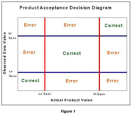
Of course, the fact that there are more potential error outcomes than correct results does not necessarily mean that errors occur more frequently than correct decisions. Figure 1 lacks a probability distribution to describe the frequency with which specific decision pairs of Actual Values and Observed Values tend to occur in each of the respective areas.

In order to generate a probability distribution, the model in equation (1) will have to be further specified. To do this, we adopt the common assumption of normally distributed random variables. Actual Product Values are assumed to be normally and independently distributed with a mean value, µ_P, and variance s_P². Measurement Errors are also assumed to be normally and independently distributed with a zero mean and a variance of s_M². The model further assumes that the actual production process the measurement process are independent of each other.

Several items are worth noting opposite these assumptions:

• The assumption of a zero mean for the Measurement Error distribution implies that the measurement process is effectively controlled to provide unbiased results.
• The independence assumptions imply that any systematic, time-related effects have been effectively removed from both the actual production process and the measurement process. In other words, the variation in each process is predominately free of "assignable cause" variation.
• The independence assumption across processes implies that the two processes are effectively unrelated.

These assumptions will allow for effective modeling of the problem. Small deviations from their exact stipulations should not have a significant impact on subsequent analysis and conclusions. Evaluating the exact effects of specific violations of these assumptions is possible, but is beyond the scope of this paper.

Given the above assumptions, the Observed Data Values will be normally and independently distributed with mean value, µ_P, and variance s_D² = s_P² + s_M². Although, it has already been suggested that Measurement Error can never be eliminated, if it were, then the implication for the more specific model would be that s_M² would be zero. In this case, the Actual Product values would be identically equal to the Observed Data Values, and the resultant probability distribution would be the familiar univariate bell-shaped normal curve (Figure 2).

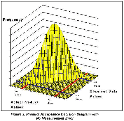
Figure 2 places the probability curve on the diagonal line intersecting at the lower left and upper right vertices of the center box in Figure 1. The probability of an occurrence in any of the error areas is zero, consistent with a perfect measurement situation.

For more information: R.K. Henderson, DuPont Photomasks Inc., Reticle Technology Center, Round Rock, TX 78664. Tel: 512-310-6409. Email: robert.henderson@photomask.com.

Source: Semiconductor Online, sister website to Medical Design Online.