How To Use Reliability-Based Life Testing Sampling For Process Validation

By Mark Durivage, ASQ Fellow

The first article in this series, Risk-Based Approaches To Establishing Sample Sizes For Process Validation (June 2016) provided and established the relationship between risk and sample size. This article will demonstrate the use of reliability-based life testing for process validation.

There are times when standard attribute and variables sampling methodologies will not provide enough useful or cost-effective information to determine if acceptance requirements have been achieved — for example, when validating the assembly process for printed circuit boards (PCBs). For these cases, reliability-based life testing techniques become useful.

Reliability-based life testing is the process of placing the "unit of product" under a specified set of test conditions and measuring the time it takes to failure. This article will present two of the three types of reliability-based life tests, with each test having two options:

• Failure-terminated
  • With replacement
  • Without replacement
• Time-terminated
  • With replacement
  • Without replacement

In a failure-terminated sampling plan, testing is concluded when a predetermined number of failures occur, while time terminated testing ends when a predetermined amount of time has passed. The ultimate goal of reliability-based life testing is to determine if the mean life (θ) requirements have been met — in other words, the minimum mean time to failure that is considered satisfactory. Additionally, these test can be performed with and without replacement of the failed units.

These tests require selecting an alpha (α) level of producer’s risk and beta (β) level of consumer’s risk. The producer’s risk α is the risk of rejecting a lot with a mean life of θ₀; consumer’s risk β is the risk of accepting a lot with a mean life of θ_1.

Start With FMEA

Before we begin, we must establish our definitions of risk and their corresponding α and β levels. These definitions can and should vary based upon organizational needs. A good place to determine the risk level is from a failure mode and effects analysis (FMEA). FMEA (design, process, user) is a systematic group of activities designed to recognize, document, and evaluate the potential failure of a product or process and its effects. FMEA uses a risk priority number (RPN), which comprises frequency, detection, and severity. The higher the RPN, the higher the risk. However, a high severity in conjunction with low probability of occurrence and high probability of detection may still necessitate the appropriate controls for high risk. Table 1 depicts an example FMEA with the associated risk levels. Once the risk level has been determined (low, medium, high), the appropriate confidence level and reliability can be selected using Table 3. Figure 1 depicts the linkage from FMEA, risk, and α and β levels.

 

Table 1: Example FMEA

 

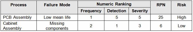
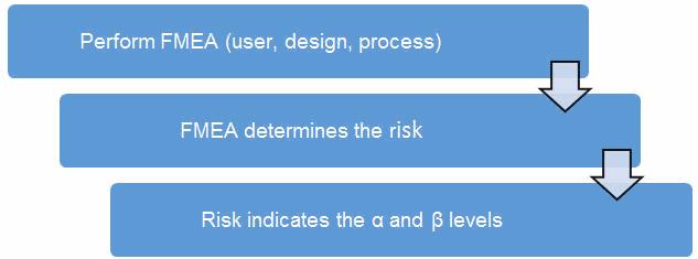
Figure 1: Risk process for determining the appropriate producer’s (α) and consumer’s (β) risk

 

Table 2 shows an example of risk level definitions with accompanying defect classifications. These definitions can and will vary based upon the product(s) and their intended and unintended uses.

 

Table 2: Example of Risk Level Definitions

 

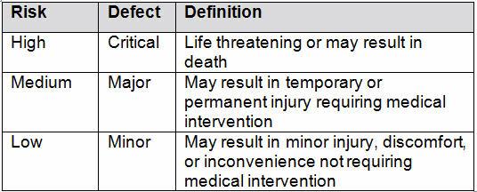
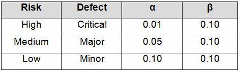
Table 3 depicts example confidence and reliability levels based upon risk. Of course, different confidence and reliability levels can and should be utilized based upon an organization’s risk acceptance determination threshold, industry practice, guidance documents, and regulatory requirements.

 

Table 3: Example Producer’s (α) and Consumer’s (β) Risk Based on Risk Acceptance

 

A Review of the Formulas Used for Mean Life (θ) Calculations

There are two formulas used when calculating the mean life (θ), depending on whether testing is done with or without replacement.

1. Formula for calculating the Mean Life (θ) when testing without replacement:

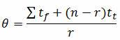
Where:

n = the number of items on test

r = the number of failures occurring during the test

t_f = total test failure time or cycles

t_t = time or cycles of last failure

Example: Ten units have been placed on test. When the units failed, they were immediately replaced. The test was terminated upon the completion of 200 hours. The failures occurred at 12, 27, 43, 110, and 173 hours (five failures total). Determine the mean life (θ):

 

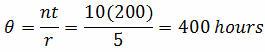
2. Formula for calculating the Mean Life (θ) when testing with replacement

Where:

n = the number of items on test

t = total test time or cycles

r = the number of failures occurring during the test

Example: Ten units have been placed on test. When the units failed, they were immediately replaced. The test was terminated upon the fifth failure. The failures occurred at 12, 27, 43, 110, 173 hours.

 

Acceptance Testing

Example: A PCB assembly process is deemed to be high risk based on the Table 1 example FMEA. Table 2 defines high risk as a critical defect that can be life threatening or may result in death, which means the process will need to be validated with an α of 0.01 and β of 0.10, according to Table 3. The validation team has decided to use a failure-terminated testing methodology.

To determine a sampling plan using a θ₀ of 1000 hours with an α of 0.01 (acceptance probability of 99%) and θ₁ of 200 hours with a β = 0.10 (acceptance probability of 10%):

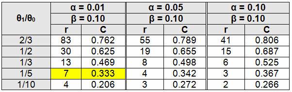
θ₁/θ₀ = 200/1000 = 1/5

From Table 4, r = 7 (Place seven or more units on test, with or without replacement, and terminate the test when the seventh  failure occurs.)

C = 0.333 (Multiply C by θ₀, in this case 0.333 x 1000 = 333 hours. If the estimate of θ upon the seventh failure is greater than 333 hours, accept the lot, otherwise reject.)

It should be noted that as θ₀ and θ₁ values become closer, the amount of testing increases exponentially. This is because it takes more data to discriminate when the values are closer to each other. Additionally, if θ₁/θ₀ does not yield a fraction contained in the table, use the next larger option. For example, if θ₁/θ₀ is 1/6, use 1/5.

The differences between using without and with replacement are:

• Testing time may increase to reach the required number of failures when testing without replacement.
• Costs of increased testing time and subjecting more units for testing when testing with replacement
• The calculation of θ

 

Table 4: Tests Terminated Upon Occurrences of Predefined Number of Failures, Without (r) and With (C) Replacement (Adapted from Quality Control and Reliability Handbook 108, Table 2 B-5)

 

Example: A PCB assembly process is deemed to be high risk based on the Table 1 example FMEA. Table 2 defines high risk as a critical defect which can be life threatening or may result in death, which means the process will need to be validated with an α of 0.01 and β of 0.10. The validation team has decided to use a time-terminated with replacement testing methodology.

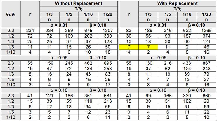
Determine a sampling plan using a 300-hour test (T) with a θ₀ of 1000 hours with an α of 0.01 (acceptance probability of 99%), and a θ₁ of 200 hours with a β = 0.10 (acceptance probability of 10%).

θ₁/θ₀ = 200/1000 = 1/5

T/θ₀ = 300/1000 = 1/3

From Table 5, n = 7 (place seven or more units on test with replacement, and terminate the test when 300 hours of testing is completed or r = 7 failure occurs, whichever is first, in this case the seventh). Accept the lot if the seventh failure did not occur when the test was terminated at 300 hours, otherwise reject.

 

Table 5: Tests Terminated Upon Occurrences of Predefined Time Without and With Replacement (Adapted from Quality Control and Reliability Handbook 108, Tables 2 C-3 and 2 C-4)

 

The main difference between using without replacement instead of with replacement is that without replacement will require more units for testing to yield the same level of protection.

Again, it should be noted that as θ₀ and θ_1, as well as T and θ₀, values become closer, the amount of testing increases exponentially. This is because it takes more data to discriminate when the values are closer to each other. Additionally, if θ₁/θ₀ does not yield a fraction contained in the table, use the next larger option. For example, if θ₁/θ₀ is 1/6, use 1/5. If T/θ₀ does not yield a fraction contained in the table, use the next smaller option. For example, if T/θ₀ is 1/6, use 1/10.

I want to reiterate that different α and β levels can and should be utilized based upon an organization’s risk acceptance determination threshold, industry practice, guidance documents, and regulatory requirements.

I cannot emphasize enough the importance of proceduralizing (documenting) the statistical methods and rationale your organization may use for process validation activities. Table 2 provides an example to document and standardize risk levels, defect classifications, and defect definitions. Table 3 provides an example to document the alpha (α) and beta (β) level requirements for process validation activities. I also recommend that validation and statistical technique procedures include the formulas as well as fully worked examples, like those demonstrated above, to provide clarity and guidance for those individuals writing, performing, executing, and approving process validation activities.

Subsequent articles in this series will provide additional how-to examples on applying risk-based sample size techniques to process validations in your organization.

 About the Author

Mark Allen Durivage is the managing principal consultant at Quality Systems Compliance LLC and an author of several quality-related books. He earned a B.A.S. in computer aided machining from Siena Heights University and an M.S. in quality management from Eastern Michigan University. Durivage is an ASQ Fellow and holds several ASQ certifications including CQM/OE, CRE, CQE, CQA, CHA, CBA, CPGP, and CSSBB. He also is a Certified Tissue Bank Specialist (CTBS) and holds a Global Regulatory Affairs Certification (RAC). Durivage resides in Lambertville, MI. Please feel free to email him at mark.durivage@qscompliance.com with any questions or comments, or connect with him on LinkedIn.

References:

1. Durivage, M.A., 2014, Practical Engineering, Process, and Reliability Statistics, Milwaukee, ASQ Quality Press
2. Durivage, M.A. and Mehta B., 2016, Practical Process Validation, Milwaukee, ASQ Quality Press
3. Durivage, M.A., 2016, Risk-Based Approaches To Establishing Sample Sizes For Process Validation, Life Science Connect
4. Quality Control and Reliability Handbook 108, Sampling Procedures and Tables for Life and Reliability Testing (Based on the Exponential Distribution), Office of the Secretary of Defense (Supply and Logistics), 1960: Washington, DC